PROFIT VBox¶
Software for the simulation and reporting of IFRS compliant Profitability after all Cost — ex ante or ex post as per single Instrument. The objective is to report the Actual Performance as per Contract, Customer, Profit Centre, Product or Segment exactly as it will be recognised in the Statement of Comprehensive Income (P&L) so that there will be only one consistent version of the truth.
Return on Equity¶
The Basel Accords define minimum Capital Requirements for all Financial Assets and thus limit the Bank’s Exposure and Business Activities based on the available Capital. Thus Capital should be optimally allocated in profitable ventures only.
PROFIT VBox will calculate the Income and the Attributable Cost of any Financial Asset or Liability in order to calculate the Return on Equity after Compensation of the Shareholders.
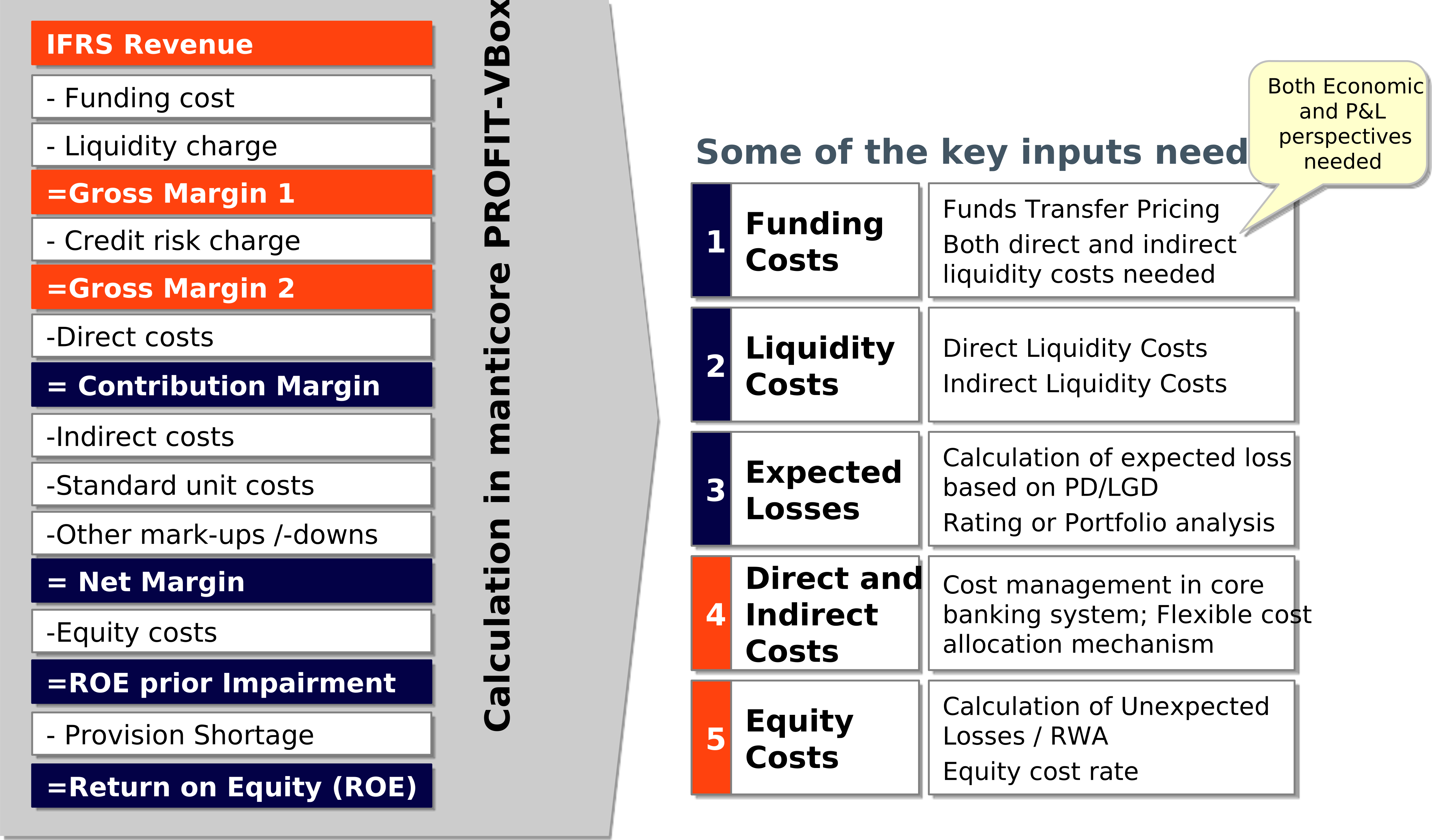
Return on Equity Calculation¶
Contract Modification¶
When a Contract is restructured on behalf of a distressed Customer in order to ease the Debt Service, then the P&L impact of this Modification will need to be recognised as a Cost (similar to a Subsidy or a partial write off). This Cost is the difference between the Book Value before Modification and the Present Value of the modified Cash Flows (discounted at the original EIR before Modification).
Measuring that Cost correctly is not an accounting formality. It determines the Carrying Amount of the Asset, the Staging of the Exposure, the Margin reported by the Profit Centre and the Funding Position carried by Treasury — and it is the only number on which a Restructuring decision can sensibly be taken.
Why the Modification Cost Must Be Measured¶
Regulatory Perspective. Where a Modification does not result in Derecognition, IFRS 9 §5.4.3 requires the Gross Carrying Amount to be recalculated as the Present Value of the renegotiated Cash Flows, discounted at the original Effective Interest Rate, with the difference recognised immediately in P&L. Three further assessments follow directly from that measurement:
the Substantial Modification Assessment, which decides between Modification and Derecognition — two entirely different accounting outcomes for the same Negotiation
Forbearance Classification, which drives Significant Increase in Credit Risk, Stage Allocation, Non-Performing Exposure reporting and the Disclosures required under IFRS 7 and local prudential rules (e.g. CBN, EBA)
Auditability, since the Day-One Loss is recomputed by the Auditor from the original Cash Flow Schedule and the original EIR — both of which must still be retrievable years later
Economic Perspective. Independently of the standard, the Concession has a Price and the Bank carries it:
it is a Subsidy to the Customer, measured as the difference between what was contractually owed and what will now be paid
unless it is quantified before the offer is made, the Restructuring cannot be compared against the Alternatives — Waiver, Moratorium, Tenor Extension, Refinancing or Enforcement
the Funding Side does not move: Treasury raised and priced the funding against the original Cash Flow Schedule, so the waived or deferred Interest Income simply does not arrive while the Funding Cost continues to accrue — a negative Margin which no Credit Report shows
Return on Equity, RAROC and Profit Centre Performance stay overstated for as long as the Cost is unrecognised, and Capital remains allocated to Exposures which no longer earn their Hurdle Rate
Measuring the Modification Loss¶
The Modification Loss is the difference between the Amortised Cost of the Contract immediately before Modification and the Present Value of the modified Cash Flows, discounted at the Effective Interest Rate of the original Contract:
The original EIR is never re-set — only the Cash Flows change. This is precisely what makes the Concession visible as a Cost, instead of disappearing into a lower Yield on an apparently new Contract.
PROFIT VBox simulates the common Restructuring Patterns interactively, each of which redistributes the Cash Flows differently over time:
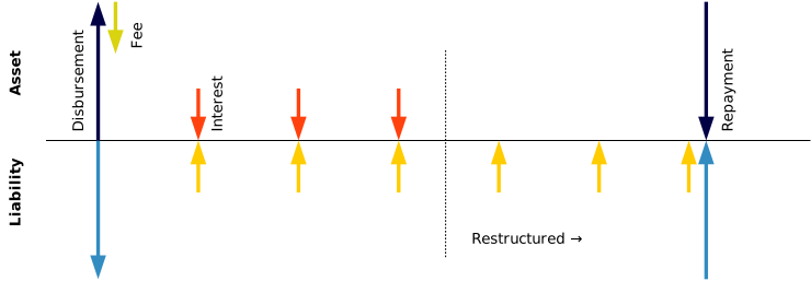
Interest Waiver¶
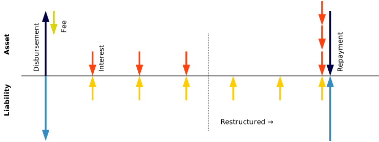
Interest Moratorium¶
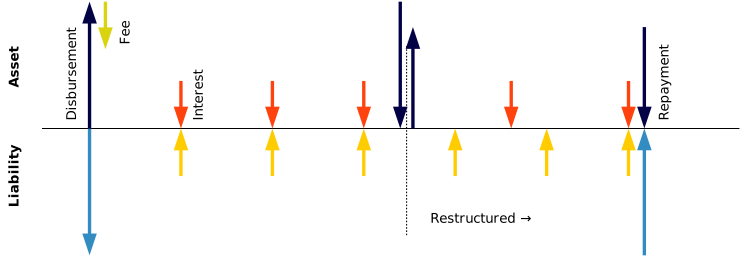
Liquidation¶
PROFIT VBox will:
generate the Original Contracts and Cash Flow Schedules before Modification
calculate the EIR and Amortised Cost (Book Value) of the Contract on Modification Date
interactively simulate the Modification (e.g. Moratorium, Waiver)
distribute the modified Cash Flows across the Original Contracts and
discount the distributed Cash Flows down to the Present Value as per Original Contract
print an Application with the Modification Details which can be authorised by the Decision Makers (alternatively, there is an Electronic Workflow)
Distributing Cash Flows across the Original Contracts¶
A Restructuring is negotiated as a package. In practice n existing Facilities — each with its own Origination Date, Currency, Collateral, Stage and, critically, its own original EIR — are replaced by m modified Schedules, where m is rarely equal to n and frequently equal to one.
Recognition, however, remains as per single Instrument. The modified Cash Flows must therefore be distributed back onto the Original Contracts by an Allocation Key \(\alpha_{j}\) before any Present Value can be computed:
Because every Original Contract discounts at a different EIR, the Allocation Key changes the total Modification Loss directly. The step cannot be approximated at Customer level, and it is the main reason why spreadsheet-based Restructuring Calculations break down as soon as more than one Facility is involved.
Amortisation under the Modified Contract¶
Recognition of the Day-One Cost is not the end of the measurement. The reduced Carrying Amount continues to unwind at the original EIR across the new Payment Schedule, so the Modification Loss is progressively earned back as Interest Income over the remaining life of the Contract.
This creates a second Amortised Cost Schedule which has to be maintained and reconciled at every Reporting Date until Maturity or Cure — on a Contract whose terms no longer match the one originally booked. In parallel, the Exposure remains flagged as forborne, and its Stage Migration and Cure Behaviour continue to be monitored against the restructured Terms.
Consequences of an Incorrect Calculation¶
Where a Modification is booked as a new Contract instead of being measured against the old one, the consequences are systematic rather than isolated:
Overstated Carrying Value — the Asset remains on the books at an amount the Customer will never pay
Unfunded Margin in Treasury — the expected Interest Income never arrives, while the Funding Cost raised against the original Schedule continues to run
Concealed Forbearance — restructured Exposures remain in Stage 1 and outside the Non-Performing Exposure and Forbearance Registers
Provisioning and Capital Shortfall — ECL and RWA are computed on an inflated Exposure Base, so the Capital Adequacy Ratio is misstated
Deferred Loss — the unrecognised Day-One Cost resurfaces later as an Audit Adjustment or a Prior-Period Restatement
Undocumented Decisions — Concessions are approved with no view of what they cost, and no record of the Alternatives which were considered
Automation and Audit Trail¶
Contract Modification is an event-driven calculation, triggered case by case and usually under time pressure during a Negotiation. Four properties of the measurement make manual processing unreliable:
The n : m Relationship — modified Schedules must be redistributed onto the Original Contracts and their individual EIRs before any Present Value exists at all
Ex-ante before ex-post — best practice is to simulate the Modification before it is agreed on, so that the Cost of every option is on the table when the decision is taken; PROFIT VBox equally supports the Calculation ex-post, after the Modification has been agreed
Amortisation to Maturity — each case creates a Schedule which must be reconciled at every Reporting Date until Maturity or Cure
Track Record and Audit Trail — each case must remain reproducible years later, including the pre-modification state, the Assumptions, the Alternatives, the Approver and the resulting Loss; the same history is the empirical basis for the Cure and Re-Default Rates which feed the ECL Model
A manual calculation produces a number nobody can reproduce. An automated one produces the same number in the Application, the Ledger and the Disclosure.
Stress Testing¶
Regulatory Stress Testing requires Banks to quantify the impact of severe but plausible economic shocks on their Credit Portfolios. PROFIT VBox implements a complete, automated Stress Testing Pipeline — from shocked Macroeconomic Covariates through to probability-weighted Expected Credit Losses and Capital Adequacy impact.
The methodology follows the Perfect Foresight approach used in ECB Supervisory Stress Tests: a defined Macroeconomic Scenario is applied to the Portfolio without Management Overlays or Mitigation Assumptions, and the resulting Credit Losses are computed deterministically through the IFRS 9 framework.
From Macroeconomic Shocks to Stressed PDs¶
The Starting Point of every Stress Test is a Macroeconomic Scenario: a set of shocked Covariates describing a plausible adverse Economic Environment over a multi-year Horizon. Typical Covariates include GDP Growth, Unemployment Rates, Interest Rates, Exchange Rates, Commodity Prices (e.g. oil), and Sector-Specific Indices.
VBox translates these Macroeconomic Shocks into Credit Risk Parameters using Satellite Regression Models that link each Segment’s Point-in-Time Probability of Default (PD PIT) to the relevant Macroeconomic Drivers:
where s denotes the Portfolio Segment and t the Projection Year. The Regression Coefficients are estimated from historical data, capturing the empirically observed sensitivity of Default Rates to each Macroeconomic Driver.
The result is a Term Structure of stressed PD PIT for each Segment and each Scenario — typically spanning 1 to 3 years — which forms the input to the Staging and ECL Calculation Engine.
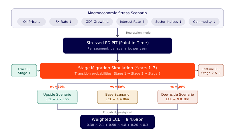
End-to-end Stress Testing Pipeline: Macroeconomic Scenario → stressed PD PIT → Stage Migration Simulation → probability-weighted ECL¶
Stage Migration Simulation¶
Under IFRS 9, the ECL for a Financial Instrument depends critically on its Stage Classification:
Stage 1 (Performing): No Significant Increase in Credit Risk since origination. Provision = 12-month ECL.
Stage 2 (Underperforming): Significant Increase in Credit Risk, but not yet credit-impaired. Provision = Lifetime ECL.
Stage 3 (Default / Credit-impaired): Objective evidence of Impairment. Provision = Lifetime ECL.
A Macroeconomic Shock changes the Probability of Default, which in turn changes the likelihood that Instruments will migrate between Stages. This migration is the primary driver of the ECL Cliff Effect under stress — as Exposures move from Stage 1 (12-month ECL) to Stage 2 or 3 (Lifetime ECL), the Provisioning requirement can increase by an order of magnitude.
VBox simulates the Stage Migration Dynamics over a 3-year Horizon using the stressed PD PIT:
Transition Matrix Estimation: For each Projection Year, VBox derives a Stage Transition Probability Matrix from the stressed PDs. The matrix captures the probability of migrating from any Stage to any other Stage (including cures from Stage 2 back to Stage 1, which become increasingly rare under stress).
Year-by-Year Propagation: The Portfolio’s Stage Distribution at each year-end is computed by applying the Transition Matrix to the prior year’s distribution. This captures the compounding effect of sustained stress — a moderate annual Downgrade Rate produces a dramatic cumulative shift in Portfolio Composition over 3 years.
Exposure-Level Staging: Each individual Exposure is assigned a Stage at each Projection Point based on its Segment’s Transition Probabilities and its individual Risk Characteristics (e.g. Days Past Due, Restructuring flags, Sector, insider-related Status).
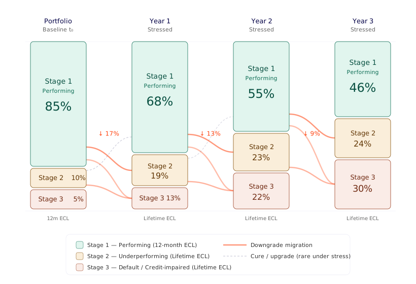
Simulated Stage Migration under a Macroeconomic Stress Scenario: progressive deterioration of the Portfolio Composition over a 3-year Horizon. Curved paths show Migration Flows between Stages; downgrade migration accelerates under sustained stress while Cure Rates diminish.¶
The diagram illustrates a characteristic Stress Pattern: Stage 1 (Performing) declines from 85% to 46% over three years as Exposures progressively migrate to Stage 2 and Stage 3. The Downgrade Flow is initially concentrated in the Stage 1 → Stage 2 transition (significant Credit Risk increase), but the cumulative effect of multi-year stress drives a substantial share of the Portfolio into Stage 3 (default) by Year 3.
From Staged Portfolio to Probability-Weighted ECL¶
Once the Stage Distribution at each Projection Year is known, VBox computes the ECL for each Exposure at each Stage:
where:
PD is the stressed Probability of Default (12-month for Stage 1, lifetime cumulative for Stages 2 and 3)
LGD is the Loss Given Default, adjusted for Collateral Haircuts under the stress Scenario
EAD is the Exposure at Default, including Undrawn Commitments and Off-Balance Sheet Items
The Portfolio-Level ECL under each Scenario is the sum across all Exposures. For forward-looking IFRS 9 compliance, VBox computes the probability-weighted ECL across multiple Macroeconomic Scenarios:
where \(w_k\) is the assigned Probability Weight for Scenario \(k\) (e.g. 30% upside, 50% base, 20% downside) and \(\text{ECL}_k\) is the total ECL computed under that Scenario.
This probability-weighted approach ensures that the reported ECL reflects the Bank’s Best Estimate of expected Losses across a range of plausible futures — as required by IFRS 9’s forward-looking Impairment Model.
Impact on Capital Adequacy¶
The stressed ECL directly affects the Bank’s Capital Adequacy Ratio (CAR) through two channels:
Increased Loan Loss Provisions reduce Retained Earnings and thus Tier 1 Capital.
Stage Migration increases Risk-Weighted Assets (RWA) as Exposures in worse Stages attract higher Risk Weights.
VBox reports the full Capital Impact Chain: pre-stress CAR, post-stress CAR, and Capital Shortfall — exactly as required by regulatory frameworks such as the CBN’s March 2026 Circular or the ECB’s Supervisory Stress Test methodology.
Why Automation Matters¶
The iterative nature of Stress Testing — multiple Scenarios, Sensitivity Analysis, Scenario Calibration — makes automation essential. VBox executes a full Portfolio Stress Run in minutes, enabling Banks to:
Sweep 10–15 Macroeconomic Scenarios to map the full CAR Impact Surface
Isolate individual Risk Drivers (Oil Price vs. FX vs. Sector Stress) to understand which factors dominate the Capital Outcome
Identify threshold boundaries where the Bank’s CAR crosses regulatory minimums
Pre-validate results against the Regulator’s likely Assumptions before submission
A manual process produces one result in weeks. An automated platform produces the understanding to make that result defensible.